
Producing H2 at a cost of £1/kg represents a threshold where it becomes a viable alternative to fossil fuels in industries like steel making, chemicals, and transport. This is based on H2’s higher heating value (HHV) of ~40 kWh/kg, meaning £1/kg H2 equates to £0.025kWh – competitive with the £0.02-0.04/kWh that gas or diesel trade at in the UK. That means even if electrolysers were free, if the energy required to produce the H2 costs over 2.5p/kWh, £1/kg H2 is impossible.
Where are we today?
Current estimates of state of the art green hydrogen production using Solid-oxide Electrolysis Cell (SOEC), with $0.05/kWh input electricity from solar PV and 9-hours of battery storage – achieve costs of ~$4/kg (£3/kg). 3x the cost that is required. SOEC’s follow the traditional engineering zeitgeist of pushing for ultra high efficiency and long-duration operation.
The thermodynamic limit (Gibbs free energy) of splitting water into H2 and O2 (via electrolysis), assuming a lossless system, is 33kWh/kg. Adding in real-world enthalpy, you get to the reverse of combustion of 39.4kWh/kg, that reflects the difference between the reversible and the thermal-neutral voltage (below). Therefore, for ease, we’ll use 40kWh/kg as the minimum input energy requirement to produce Hydrogen throughout this analysis.

There are 3 types of electrolyser architecture currently being utilised at scale:
- SOEC – High-temperature with ceramic electrolyte.
- PEM – Low-temperature with solid polymer electrolyte.
- AWE – Low-temperature, liquid alkaline electrolyte.
Within any architecture, there are 2 main interdependent variables we can influence:
- Efficiency – how much electrical energy do we need to deliver to drive the non-spontaneous reaction?
- Capex – how much does the system itself cost? Electrodes, catalysts, gaskets, membranes, BoP etc.
If we are to drive towards the cheapest Levelised cost of Hydrogen (LCOH), our main aim is to be architecturally agnostic, focussing entirely on identifying which variable we can influence to the greatest degree to reduce cost.
For example, if we were focused on increasing efficiency further for SOEC to achieve £1/kg H2, would that require a dramatic cost reduction in Iridium? Is this possible and scalable for one of the rarest elements on earth with annual production volumes of a few tonnes exclusively in geopolitically unstable Russia and South Africa?
For the last 50+ years, with energy costs stubbornly high in the range of £0.1-0.5/kWh, reducing capex wasn’t a priority – rather maximising efficiency to minimise energy consumption. Efficiency gains have primarily manifested in more extreme operating conditions (pressure, temperature), more exotic electrode materials and coatings (nano structures), and more complex electrode morphologies and chemistries (foams, hydrophilicity tuning etc).
While improved efficiency has taken us from the clunky AWE’s that produced liquid hydrogen for the V2 rocket and Submarines in WW2 to almost thermodynamically perfect SOECs, they have been accompanied by substantial increases in capex:

Whilst R&D to increase efficiency continues, we can’t argue with the HHV of 40kWh/kg of H2 requiring energy input of <2.5p/kWh. How cheap is our input energy?
What is the cheapest form of energy in the world?

Solar has one of the fastest learning rates of any technology in history, named Wrights Law, dropping by between 20-30% for every doubling of production, rivalled only by semiconductors (Moores Law). Specifically, this learning rate has been 20.2% for the last 48 (!) years, and >40% since 2008, resulting in a 95% drop in solar cost in the last 10 years, roughly 12% every single year.
This learning rate makes £0.01/kWh DC electricity a reality with £300/kW off-grid solar in locations with >1200kWh/kWp. This isn’t the future, this is now.

It’s worth noting that solar didn’t get this cheap by chance. Solar is a mechanised learning-rate machine, predicated on a few core tenets:
- Speed of iteration
- Designs that are modular and replicable quickly, iterate quicker and encourage a large amount of small changes, dynamically. If your production is flexible enough to quickly update design changes weekly based on new learnings directly onto the production line, designs mature rapidly and drop costs further and faster.
- Free markets
- If you’re producing a product in a free market, there is a drive to ever decrease pricing to win more of the customer base (and survive). A solar panel is a commodity good where every design is 95% the same as every other design. As such, manufacturers aggressively reduce costs to win business, otherwise they’ll die out. To reduce costs is to stay in the game.
- Simplicity
- If designs are simple, and robust, they form a clearer path to go from 10’s and 100’s to billions produced. If we’re having to invent new processes to cut titanium alloys like those that were required during the SR71 production, we’re likely going to be hamstrung to produce millions of units.
- Robust supply chains:
- No rare earth metals or anything that can cause a vulnerability in the supply chain. Tesla has removed 75% of silicon carbide (amongst other reductions) from their production over years of iteration to rapidly scale production and decrease costs further.
A high-learning rate can be used to describe how Tesla’s became cheap enough to compete with the petrol/diesel incumbents. They vertically integrated all manufacturing to have huge ability to reduce costs on all components, piggybacked on the already fast >20% learning rate of batteries, and scaled production from 1000 cars / year with their Roadster to 10’s m’s cars a year in a ruthless automotive industry that threatens bankruptcy but rewards continual cost reductions with an ever larger customer base.
In contrast, these factors also explain why current Nuclear power plant designs, because of their complexity, large unit scale, and fragile supply chains, are extremely expensive and unlikely to drop in cost until they move closer to the factors that drive a learning-rate.
Which Electrolyser architecture should we use with the cheapest energy in the world to produce £1/kg H2?
If we take the £0.01/kWh input cost above as an anchor, and plot solar energy as an input (£0.1/kWh down to £0.005/kWh) to electrolyser capex (from £1 to £500/kW) and performance (from 40kWh/kg to 100kWh/kg) against LCOH, you get something like this:

What this graph shows is that we’re able to achieve <£5/kg with various combinations of input cost, capex, and efficiencies. Naturally, the cheapest H2/kg will be a combination of the best performance + lowest capex + lowest cost of energy (bottom-rear-right of the graph), but this is largely an impossible reality.
Interestingly however, if you move forward from the back-right corner with 40 kWh/kg efficiency, and continuously decrease efficiency towards the front-right corner with 100kWh/kg efficiency – you’re still able to maintain production costs <£5/kg H2 if energy input costs remain low. This demonstrates that when energy input costs are negligible, H2 production costs cease to be sensitive to efficiency gains.
We can apply this to a practical scenario by using £0.01/kWh input cost to 3 different electrolyser architectures (ignoring operational life, opex, and assuming BoP is factored into the capex), we get something like this:

| Technology | Electrolyzer CAPEX | H₂ Produced (kg) | Energy Cost (£/kg) | Total H₂ Cost (£/kg) |
|---|---|---|---|---|
| Solid Oxide | £4000/kW | 300.00 kg | £0.40/kg | £13.73/kg |
| PEM | £1000/kW | 266.67 kg | £0.45/kg | £4.20/kg |
| AWE | £200/kW | 218.18 kg | £0.55/kg | £1.47/kg |
The graph shows £/kg H2 on the left-hand Y axis, and aggregate H2 output in kg to the right-hand side. This agrees with the earlier 3D scatter graph, showing despite larger absolute H2 output per kW (right-hand Y axis) with higher efficiency electrolysers, the increased output is still not enough to amortise the higher capex when energy costs are near zero. Therefore, counterintuitively, when energy input costs are near zero, you need to use more energy to produce a cheaper end product.
This sensitivity bias to input energy costs only occurs for technologies where capex drops at a greater rate than its associated efficiency decrease. This alters the % of total deployed cost:

How fast do we need to decrease capex?
The larger the decrease in capex for every 1kWh of performance loss, the cheaper H2 will be produced. In other words, there needs to be a superlinear scaling coefficient between efficiency and capex.
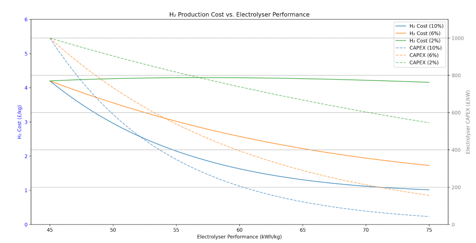
The above graph shows £/kg H2 on the left-hand side Y axis, and % capex reduction on the right-hand side Y axis plotted against electrolyser performance on the X axis. The graph describes the relationship between capex and efficiency for the PEM electrolyser numbers from earlier, £1000/kW capex and 45 kWh/kg efficiency, and how a fixed capex reduction by either 2%, 6%, or 10% for every 1kWh of performance loss influences £/kg H2.
The outcome is that any capex reduction >2% for every 1 kWh performance loss improves £/kg H2, all the way to 10% where you slip into <£1/kg H2 with £72/kW capex and 75kWh/kg efficiency. These are just indicative numbers and can be way more aggressive for lower-efficiency architectures like AWE. This again shows that any further gains in electrolyser efficiency are actually counterproductive to cheaper H2 if accompanied by capex increases, and instead the focus should be entirely on using as much cheap energy as possible.
As energy input costs continue to decrease, there is reduced requirement to continue R&D of expensive materials and electrochemistries. The development focus will instead flip to manufacturing and vertically integrating low efficiency, low capex components, essentially trading off efficiency for capex reductions using the above graph as a guide. In other words, if we are to achieve £1/kg H2 at scale, the way electrolyser manufacturers are currently set-up to drive towards the bleeding edge of innovation to achieve more efficiency, is backward.
Where is the cheapest energy on earth?

Taking this irradiance map and starting with a £300k/kW deployed off-grid solar cost, with a 10%/yr cost decrease through learning rate applied to different irradiance levels, yields the graph below.

Though riding the solar learning rate to cheaper energy is now a strong bet, we can also cheat the system by heading closer to the equator, and “buy” years of learning rate.
For example, it won’t be until 2030 that we receive £0.009 kWh solar cost in the UK at 1000kWh/kWp from the graph, but is already readily available in areas of Italy (1300 kWh/kWp), Spain (1400 kWh/kWp), Greece (1500 kWh/kWp), even cheaper in Australia at ~ 2000kWh/kWp.
However, the utilisation of that power becomes a constraint with intermittency of solar. How sensitive is LCOH to continuous 24 hour operation vs intermittent operation?
The graph below takes the same solar deployed cost of £300/kW (£0.3/W), £200/kWh battery cost, a clear-sky irradiance model yielding 1200 kWh/kWp annually, and a fixed load to determine what it would cost to power that load for a set number of hours per day:

In the first 0-4 hours of operation you’re covered by cheap solar, followed by a mix of solar overbuild and small-scale battery storage, before you have to invest heavily into large-scale battery back-ups. In essence, once power demand is offset from production, you rapidly pay for it.
This motivates to produce H2 only when the sun shines to drive costs down further, with the pareto optimum being to run for 3-4 hours/day where you strike the balance between getting just enough production spread over your capex without incurring the heavy cost of battery support.
What about compression, storage and transport?
What intermittent production ignores is the end utilisation of that molecule. H2 is notoriously difficult to store and transport, even NASA’s Artemis struggles. Whilst we have assumed BoP is loaded into capex calculations, a large % of LCOH is often derived from compression equipment, distribution equipment, purity/polishing, drying and various other peripheral infrastructure. The 3 core variables that drive up the end-utilisation of H2 are travel distance, compression and storage.
We can add a tapering cost equation to get an idea of how sensitive LCOH is to those variables using the following inputs.
- Distance
- Distance_baseline = £0.5 (cost per segment)
- Segment_size = 100 miles
- Pressure
- Pressure_baseline = £0.25 (cost per segment)
- Segment_size = 10 bar
- Storage
- Storage_baseline = £0.25 (cost per segment)
- Segment_size = 10 days
There is also a 0.7 decay factor added, meaning that for every segment jump (e.g 100 to 200 miles), It will cost 70% less than the prior segment. This is to reflect the significant upfront investment for any compression, storage or transport irrespective of actual magnitude of those operations. Put together, the graphs look like this:

If we apply those cost penalties into the following scenarios, assuming a starting point of £0.5/kg H2:
- Scenario 1: Travelling 500 miles from production, with 100 bar compression and 60 days of storage
- Scenario 2: 100 miles traveled, 50 bar compressed and 30 hours storage duration
- Scenario 3: Assumes in-situ utilisation, 10 bar compression and no storage.

| Scenario | Distance Contribution (£/kg) | Pressure Contribution (£/kg) | Storage Contribution (£/kg) | Total Additional Cost (£/kg) | Total Cost (£/kg) |
|---|---|---|---|---|---|
| Scenario 1 | 2.773 | 1.620 | 1.471 | 5.863 | 6.363 |
| Scenario 2 | 1.000 | 1.387 | 1.095 | 3.482 | 3.982 |
| Scenario 3 | 0.000 | 0.500 | 0.000 | 0.500 | 1.000 |
Whether the starting points or decays are accurate to all operations is partly irrelevant, as pretty much any travel, storage or compression removes the ability to achieve <£1/kg H2. In scenario 1, the distance contribution is 5x that of the base H2 cost alone.
This discounts the economic feasibility of using Hydrogen in high-pressure industries like transport and aviation, or in use-cases where production and consumption are separated by anything more than a pipe. On the flip side, this offers huge benefits for immediate in-situ production and utilisation at low pressure for industries like chemicals to benefit from much lower LCOH.
At Rivan Industries, we produce millions of litres of extremely cheap green H2 that we convert almost immediately to a larger, more utilitarian molecule in CH4 that is distributed in the grid to decarbonise heavy industries. We wrote about the last 12 months of R&D here on our quest to produce the cheapest H2 and capture the cheapest CO2 on the planet, and are hiring amazing engineers to make it happen.
How does this all fit together?
The above analysis should tell us that thermodynamics don’t agree with the path of continual R&D investment into more efficient electrolysers when energy is almost free. Instead, the following approach is more favourable:
- H2 production requires at least 40 kWh/kg energy, so to achieve <£1/kg H2 you must have energy less than 2.5p/kWh even if your electrolyser is free.
- The cheapest energy in the world is off-grid solar PV. Solar’s incredible learning rate can be accelerated further by moving closer to the equator to buy years of cost reductions.
- With ultra-low cost energy input, LCOH favours low-capex, low-efficiency electrolyser architectures – in direct contrast to the market and the last 50-years of R&D.
- To maintain a low LCOH, production must follow intermittent solar, not continuous production, accompanied by in-situ, low pressure utilisation.
Combining the above, it becomes a race to how fast we can reduce electrolyser capex, whilst maintaining some degree of performance to chase solar’s incredible learning rate:

The £1/kg H2 isn’t a distant dream if we rethink the framing of the problem. Since H2 will always abide by the laws of thermodynamics, and that energy intensity is really just a factor of energy cost, we must follow the energy.