
We need to capture CO2 from the sky for <£10/tonne to make a real difference, requiring a 97% drop from where we are today at ~£300/tonne, and do so at 24,000x the scale of our collective 50,000 kt/yr capacity to capture the 1200Gt that are now in the sky above the ~350ppm level. How are we going to do that?
The optimum pathway for DAC is yet to decided, but the physics are set:
\[
\Delta G = RT \ln\!\left( \frac{P_{\mathrm{CO_2,captured}}}{P_{\mathrm{CO_2,air}}} \right)
\]
Where:
R = 8.314 J/mol
T = 298 K
PCO2,air = 420 ppm (Concentration of CO2 in the air)
PCO2,captured = 1 atmP (Pressure of pure CO2 once captured)
What this really translates to is that PCO2,air is extremely dilute (0.042%), it takes a lot of of energy to increase it’s concentration to 1,000,000ppm (100%), pCO2,captured. Specifically, to separate 420ppm of CO2 from air at atmospheric pressure, it takes 19.4kJ/mol CO2. Once we have it concentrated, we can store it indefinitely, or we add further energy to pull it back out and use it for a given process. To get it back out of the capture medium, it works out at somewhere between 70 – 140 kJ/mol CO2, depending on the different binding mechanisms (from physisorption to covalent bonding) and the regeneration process (thermal or pressure swing). These are the minimum theoretical energy requirements – and don’t take into account the irreversibilities of side reactions, heat losses, pressure drop, and limitations in the reactions.
This gives us an thermodynamic limit of somewhere between 60 – 200kJ/mol, which equates to between 0.4 – 1.3 kWh/kg. To put that in perspective, the average electrical price in the UK is 25.7p/kWh, meaning 1 tonne CO2 on the high-end of that range via DAC would cost >£300/tonne just for the power input, not including anything else. We’re going to have to think about this differently!
Ever since the industrial revolution, we’ve been adding CO2 to the air at a steadily increasing pace:
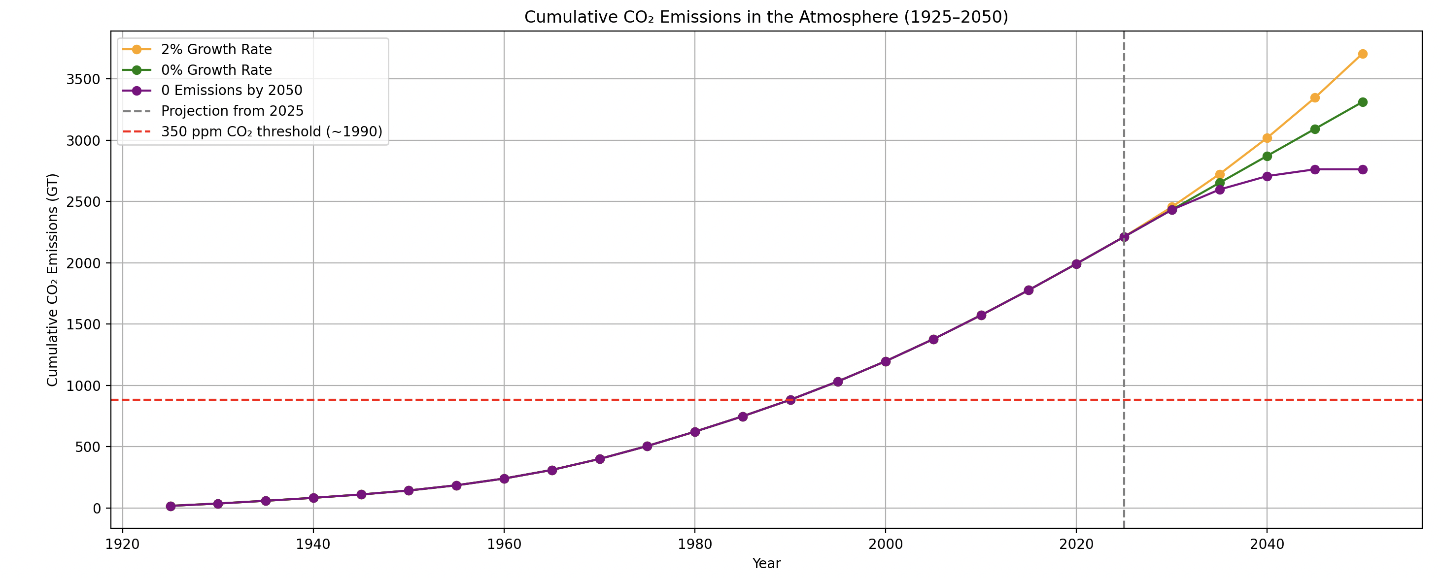
The grey vertical dotted line to the right hand side of 2020 represents where we are today with roughly 2200Gt of CO2 in the atmosphere (this focuses on just CO2. The numbers are >3000Gt if you take into account all GHGs), equating to ~ 420ppm in the air. The red horizontal dotted line marks the “safe” ppm level of 350ppm in the air where life can function as normal without any adverse effects. We blew past that in the early 1990’s, having since added >1000Gt to the sky. Therefore, we have roughly 2200-1000 = 1200Gt of CO2 to remove from the sky if all future emissions stopped today.
3 options extrapolated from today. The yellow line represents our current rate of ~ 2% per year growth rate in CO2 emissions, driven by ever larger energy requirements from data centres, construction, and travel. The green line represents a 0% growth rate, where we’re still contributing to the absolute Gt of CO2 in the sky, but not at a relatively growing rate per year. The purple line represents what Rivan is hellbent on achieving, where those emissions stagnant gradually over the next 25 years, stalling the growth of the CO2 cloud in the sky and buying us time to figure out how to pull down remaining 1200Gt. The trick is to do so cheaply without crushing GDP.
The largest operating DAC project in the world is The Climeworks Mammoth plant, capturing ~ 36,000 tonnes/yr, with Carbon Engineering’s planned 500,000 tonnes/yr Stratos project aiming to get live in 2025/6. The IEA estimates we capture around 0.5Mts (500,000 tonnes) as of today, forecast to rise to ~ 10Mt by 2026 (!), but with only 500,000 of the 10m under construction as of today:
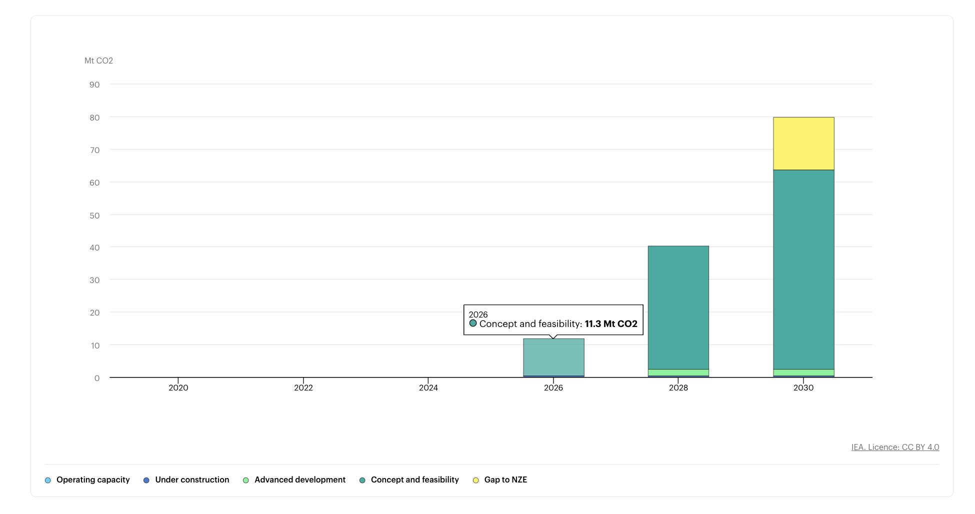
This shows we need to speed things up! Not just faster, but cheaper. “Cheap” in this instance means at a threshold where even the worst emitters can afford the £/tonne cost of CO2 capture on the profit they make per tonne of CO2 emitted, . This graph represents different sections profit/tonne of CO2 emissions (Y axis) vs aggregate CO2 emissions (X axis):
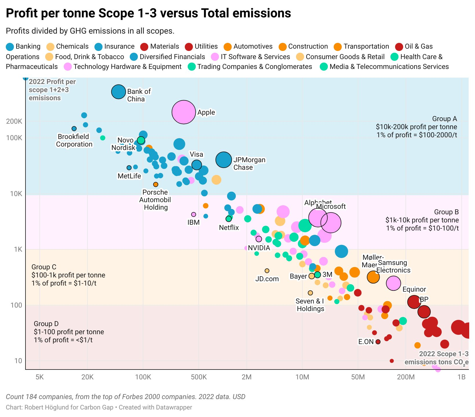
What this tells us is that large Oil & Gas majors in the bottom right have roughly $1 of profit /tonne of CO2 emissions to play with, so couldn’t ever pay the $100/tonne target price point that DAC is often built on. Since the worst emitters have the highest sensitivity to $/tonne, we’d need to get closer to $10/tonne to start to have real impact. For ease, £/$ will be interchanged during this blog as some of the data is only available in USD vs GBP.
We need to increase scale, reduce price, and do so fast. What are the options?
Architecture
Regardless of how you capture CO2 from the air, you’re always battling 2 core areas – capture efficiency and regeneration efficiency. Capture efficiency is dictated by how low the Gibbs free energy is to drive the CO2 towards equilibrium with your sorbent, whilst regeneration being the energy required to get it back to equilibrium in it’s original state as a single gaseous molecule.
Here are the most commonly used DAC pathways and their respective thermodynamics:
| DAC Architecture | ΔG capture (kJ mol) |
Regeneration ΔH (kJ mol) |
Thermodynamic Limit (kWh / CO2) |
Capture Mechanism | Regeneration Mechanism | Real-world Performance (kWh CO2) |
|---|---|---|---|---|---|---|
| Zeolite / MOF | 20.4 | 43 | 400.4 | Physisorption / Chemisorption | Temperature-Swing Adsorption | 1250 |
| Amine Solvent | 22.1 | 81.5 | 653.8 | Chemisorption | Temperature-Swing Absorption | 1450 |
| KOH Loop | 20.4 | 138.2 | 1001.3 | Chemisorption | Temperature-Swing | 1125 |
| Ca(OH)2 | 20.4 | 178.6 | 1255.7 | Chemisorption | Temperature-Swing | 1638 |
Plotted, this looks something like:
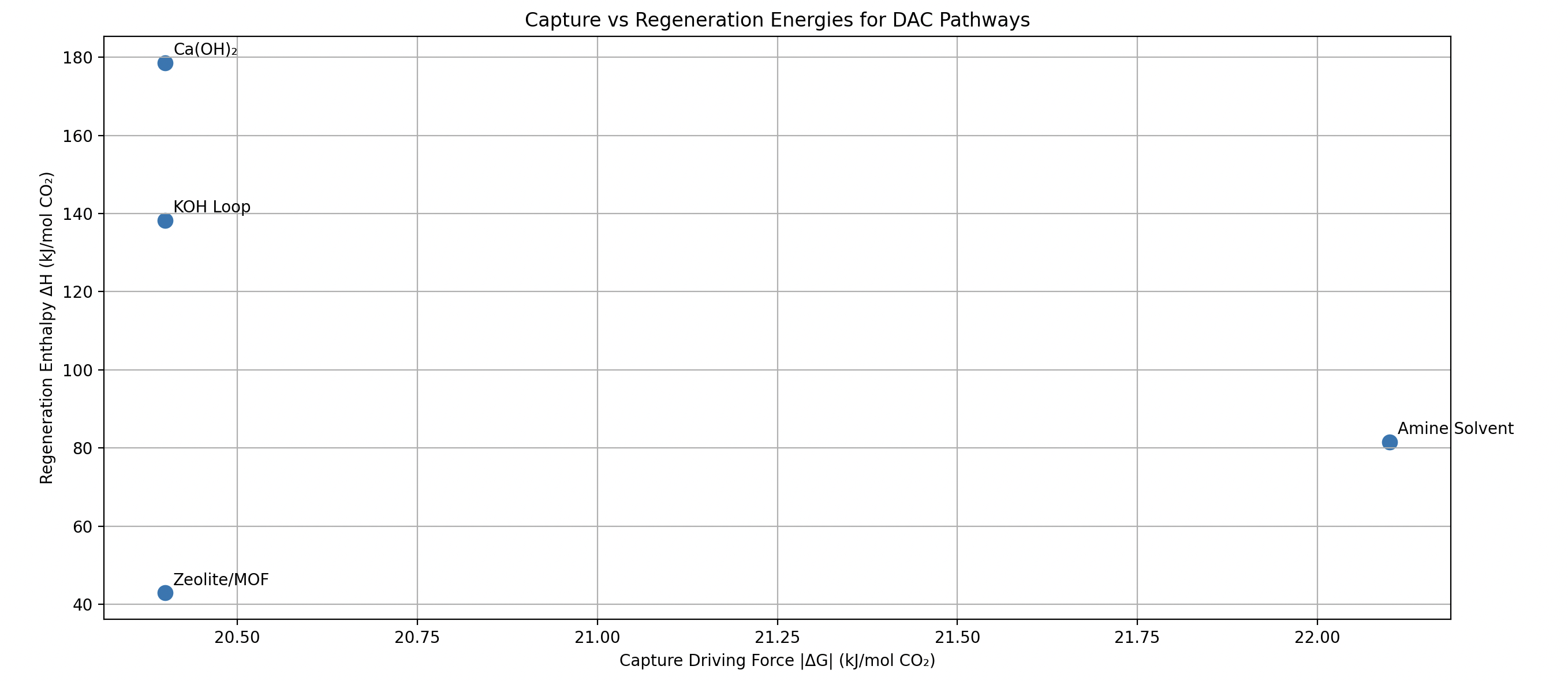
On the surface, there isn’t much difference between capture energy requirements (X axis). At 400 ppm, all pathways are primarily limited by the entropy of separating dilute CO2 from air. The theoretical minimum ΔG (~19.38–20.4 kJ/mol) depends on CO2 concentration and temperature, not the capture medium itself.
These numbers clearly lack a reality factor that takes into account all losses in the process. What is the current state-of-the-art in DAC in the real world?

References: Climeworks, MOF4air, Removr, Heirloom, Carbon Engineering.
These numbers are shaky. It’s difficult to get a good view of the facts when we’re blurring both commercial vs academia, scales/sizing, and reality vs modelled results. Lots of DAC companies aren’t incentivised to share their real £/tonne CO2 cost, and lots of purchasing deals are opaque with the details. Instead, we can reason from the ground-up using the thermodynamics from earlier.
Firstly, we can take a stab at the individual costs that make up each architecture for a 1kg/day system. These costs are high-level and assume almost perfect performance, neglecting the detail required for full system operation, cycling schedules, material degradation and the like. However, if we take £0.05/kWh as input energy, and use the thermodynamic limits above for kWh/tonne, we get something like this:
| Architecture | Component | Low (£) | High (£) | Notes |
|---|---|---|---|---|
| Solid Amine | Sorbent cartridge (PEI/Si) | 1 500 | 2 000 | Assuming 5kg (here), Replaceable every 6–12 months Polyethylenimine on silica gel Maximum uptake: 1–3 mmol/g Working capacity: 60% (1.2 mmol/g) Mass required: 53mg/g / 1000 = 1.9 kg Cycling: 2 beds (1.9*2) = 3.8kg (+ buffer) Total mass = 5kg |
| Air-contactor module | 600 | 1 000 | Packed-bed housing; 80–120 °C thermal swing | |
| Fans / blowers | 200 | 400 | 100–200 m³ h⁻¹ air flow | |
| Heater elements & piping | 200 | 400 | Regeneration 80–120 °C | |
| Heat exchangers | 200 | 400 | Recuperative or direct-contact | |
| Controls & instrumentation | 200 | 400 | Valves, sensors, PLC | |
| Skid / foundations | 200 | 400 | Skid, piping, foundation | |
| CapEx/kW | £4150 |
| Architecture | Component | Low (£) | High (£) | Notes |
|---|---|---|---|---|
| KOH + Ca Loop | KOH absorber & precipitator | 1 000 | 2 000 | Cross-flow tower / cooling tower structure |
| CaCO₃ calciner (kiln) | 1 000 | 2 000 | Small-scale furnace (muffle or cylinder); regeneration ≈ 900 °C | |
| Solid-handling (conveyors) | 500 | 1 000 | For CaCO₃ / CaO transport | |
| Fans / blowers | 200 | 400 | 100–200 m³ air flow | |
| Controls & instrumentation | 200 | 400 | pH control, level sensors, PLC | |
| Hydrator | 200 | 400 | Mixing / water-dosing equipment | |
| Skid / foundations | 200 | 400 | Foundations, piping, skid | |
| CapEx/kW | £6200 |
| Architecture | Component | Low (£) | High (£) | Notes |
|---|---|---|---|---|
| CaO Looping | Sorbent (CaO) | 3 | 6 | Assuming 0.5g/g working capacity with buffer |
| Kiln / calciner | 1 000 | 2 000 | Lab-scale high-T furnace; regeneration ≈ 900 °C | |
| Powder-handling system | 250 | 500 | Conveyors, fluid-bed, etc. | |
| Gas/solid contactor | 100 | 200 | Provides surface area for carbonation | |
| Fans / blowers | 200 | 400 | 100–200 m³ air flow | |
| Hydrator | 200 | 400 | Mixing / water-dosing equipment | |
| Skid / foundations | 200 | 400 | Foundations, piping, skid | |
| CapEx/kW | £3356 |
| Architecture | Component | Low (£) | High (£) | Notes |
|---|---|---|---|---|
| Zeolite | Sorbent cartridge (zeolite / MOF) | 2 500 | 5 000 | Assuming Zeolite 13X Maximum uptake: 1–2 mmol g Working capacity: 0.75 mmol g (33 mg g) Mass required: 33mg/g / 1000 = ~30kg (+ buffer) Total mass: 50kg |
| Gas/solid contactor | 500 | 1 000 | Packed bed | |
| Vacuum pump & plumbing | 200 | 400 | Central vacuum manifold for regeneration | |
| Fans / air movers | 200 | 400 | 100–200 m³ airflow | |
| Heat exchanger | 200 | 400 | Recuperative heat management | |
| Controls & instrumentation | 200 | 400 | Valves, pressure sensors, PLC | |
| Skid | 200 | 400 | Skid, framing, electrical & vacuum piping | |
| CapEx/kW | £8150 |
The capex will also appear inflated because of the lack of economies of scale with a 1kg/day set-up. That said, you can get an idea of £/tonne CO2 using ((Input energy cost * efficiency) + Capex))/total production volume:

It would make sense that Zeolites have the lowest £/tonne CO2 at £60, based on the thermodynamics being far more favourable. However, if our aim is to drive to prices <£10, we need to know the make-up of total cost to understand which levers we can pull to reduce further:

This tells us that Zeolite/MOFs are overwhelmingly Capex sensitive (~70% of levelised cost), whereas CaO in the bottom right is majority Opex sensitive (~60%). If both of these architectures are delivering £60-100/tonne CO2 based on their thermodynamic limits, once you add in real world inefficiencies we’re likely looking at double those costs. Therefore, we’re still over an order of magnitude away from our cost targets. To drive cost further down, we either decrease capex for high efficiency systems like Zeolites, or increase efficiency for lower efficiency systems like CaO….right?
Capex vs opex
To decide which avenue to go down, we need to know which variable (1) has the most impact and (2) we have a large influence on?
To model this, agnostic of architecture, we’ll plot a range of energy input costs from £0.005/kWh (extremely cheap!) to £0.1/kWh, a range of efficiencies from 500kWh/tonne through to 5000kWh/tonne, and a range of capex from £250/kW to £10,000/kW.
The calculation works in the same way in the earlier calculation to get £/tonne, by assuming 24 hour operation for 10 years for a 1kW system (1kW * 24 * 365 * 10 = 87,600kWh), multiplied by the efficiency to get a total production value in tonnes, divided by the capex and energy input costs. Put together, you get this:
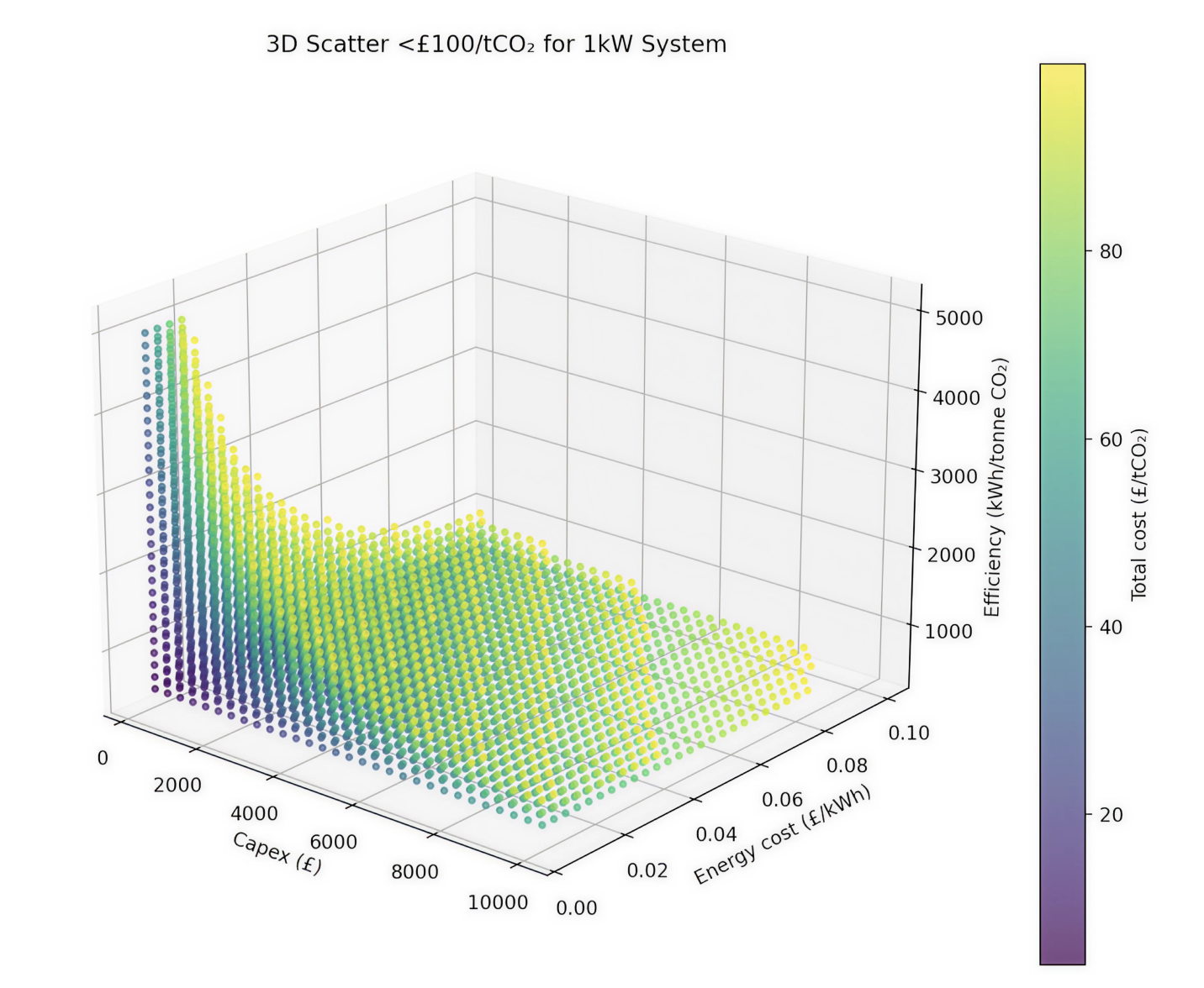
Firstly, we can immediately filter out the “impossibles”, where a combination of high-efficiency, low capex, and low energy input costs aren’t baked in reality. This counts out scenarios like 1000kWh/tonne at £250/kW cost with £0.005/kWh input energy. However, once they are removed, we can see the cheapest £/tonne CO2 is concentrated on the low capex and cheap energy region to the left hand side in purple, with efficiency playing less of an impact. This tells us that when energy costs are low, capex becomes incredibly important and favours lower efficiency, cheaper architectures – counter to the high-efficiency and high-capex design direction of modern engineering.
Specifically, the graph shows that even if we plug in extremely cheap energy to an efficient DAC system (e.g a 1000kWh/tonne system that costs £10,000/kW – see bottom right in the graph), it’s not very sensitive to the low energy costs, as a large % of overall cost is already baked into the capex, and drives up £/tonne CO2 costs. This reflects the pie charts discussed above where Zeolites/MOFs made up a large % of overall capex, and thus any reduction in opex wouldn’t really make much difference. This principle is even clearer when you cut down the outputs further to <£50/tonne, stripping away another ~ 50% of the above combinations:

This immediately removes almost any architectures where high-efficiency has a high-capex prerequisite, such as Zeolites/MOFs or amines, until we can make them at scale cheaply. Instead, this favours low capex and low(er) efficiency architectures such as CaO, where they are much more sensitive to the falling cost of energy. Why? Because a large chunk of overall costs is energy input. Why? Because it’s thermodynamically unfavorable because of immense energy requirements for regeneration, but uses cheaper components and equipment. Some of these scenarios may still be beyond possibility where you simply can’t get capex far enough down whilst maintaining some level of efficiency, but the top-left red arrow represents a more plausible opportunity with a combination of:
- Ultra low efficiency: ~5000kWh/tonne CO2
- Ultra low capex equipment: ~£250/kW
- Ultra low input power costs: ~£0.005/kWh
Overall, this analysis shows that further optimisation for higher efficiency can’t get to the prices required until capex is significantly reduced. On the other hand, it shows that often overlooked architectures that are far worse from a thermodynamic perspective offer a clearer path to cheaper carbon capture because of their low capex and sensitivity to low energy input costs. How can we bring the combination of low capex, low efficiency and low energy input costs to life?
Where is the cheapest energy in the world?
We’ll cover the core principles here, but for a more comprehensive breakdown of cheap electricity, read our recent £1/kg H2 blog. If we need to get to £0.005/kWh electrons, how far away are we if we anchor on standard electrical prices across the world today?
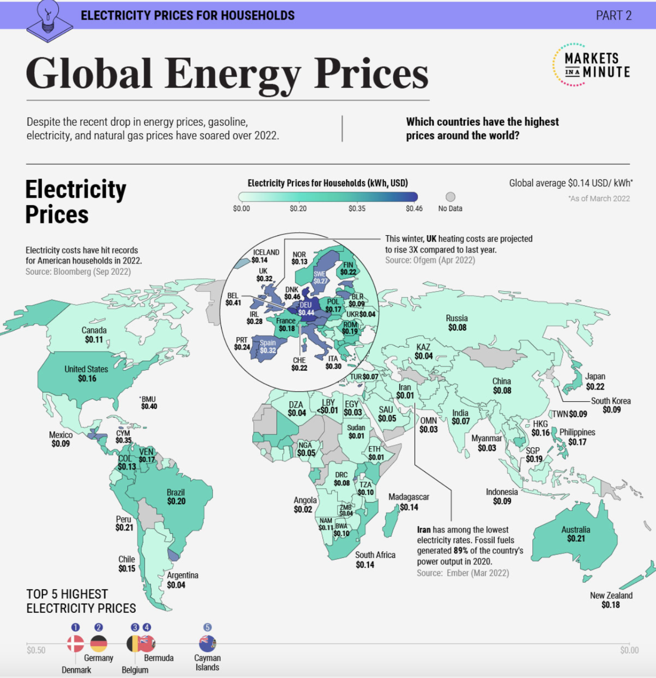
Some areas of Africa and the Middle-East get close to £0.03/kWh, but that’s still 6x higher than what’s required in our analysis above. Why is that? That cost is a bundle of everything from distribution costs and operator margins, to policy requirements and network infrastructure costs. To gain access to cheap electrons, you need to remove all barriers on their way to you that would otherwise increase the cost of their transport. Usually, electrical distribution looks something like this:
Power Generation (e.g., Power Plant)
v
High Voltage Transmission Lines (e.g., 275kV – 400kV)
v
Step-Down Transformer (Grid Substation – reduces to ~132kV)
v
Medium Voltage Transmission (e.g., 33kV – 66kV)
v
Primary Substation (Step-down to ~11kV)
v
Low Voltage Distribution (11kV → 400V transformer at local substation)
v
Low Voltage Network (Three-phase 400V or single-phase 230V)
v
Service Line to Home (via Meter + Main Breaker)
v
Consumer Distribution Board (fuse box)
v
Individual Circuits (Sockets, Lights, etc.)
v
Home Appliance (e.g., toaster, fridge, etc.)
This racks up costs. Instead, to find energy costs closer to those required, we need to remove as many stages as possible, and get as close to the generation of the electron as possible. The closest we can get to that today is DC off-grid solar.
This extreme price decrease is achieved because solar PV pricing is currently dropping at an eye-watering rate of ~ 12%/yr, averaging >20% for the last 48 years straight (!). Even if we assume that somehow the wheels of motion of a capitalism driven learning rate grind to a halt, or even spin in reverse for a few years and double the cost of panels, we’d still be looking at £0.01/kWh, 3x cheaper than the cheapest electrons in the map above.
To model this, we can use a £300/kW deployed off-grid solar cost, with a 10%/yr cost decrease through learning rate, applied to different irradiance levels across the world (e.g closer to the equator = more sun!), to get this graph we described in our £1/kg H2 blog:

This shows that off-grid solar energy in areas near the equator now already achieve <£0.005/kWh DC pricing, driving towards the almost unthinkable £0.001/kWh over the next 10 years.
If one of the 3 core components of <£10/tonne CO2 is input energy <£0.005/kWh that is already viable from DC off-grid solar, how can we make sure the ultra capex is also achievable?
How to drive down capex
Sensitivity to falling energy input costs only function when there is an even more extreme cost reduction in capex. In other words, you need to be able to drop the capex faster than the loss of performance (e.g using more energy), otherwise £/tonne CO2 will go up.
To get an idea of how fast we need to drop capex, we can model the same parameters as the scatter graph above, assuming an efficiency range of 1000kWh/tonne CO2 to 5000kWh/tonne CO2, and capex from £100/kW to £5000/kW. From there, we can add a fixed capex reduction for every 0.25kWh/kg drop in performance, ranging from 5% to 20%. For example, if we drop capex by 20% from £5000/kW to £4000/kW, efficiency would drop by 0.25kWh, what happens to the £/tonne CO2 cost? Everything in the following graph has been modelled on the kWh/kg level for higher fidelity:

The blue line shows that an initial capex reduction of 5% for every 0.25kWh performance loss actually increases £/kg CO2, driving us to higher capex reduction rates. The orange line starts to get to cheaper £/kg CO2 with a 10% capex reduction, but not to the extent where the outcome achieves the desired £10/tonne CO2, finishing around £50/tonne at 5kWh/kg. It’s not until you drop capex aggressively by 20% for every 0.25kWh/kg performance loss, the green line, that you dip <£20/tonne with an ending capex of £274/kW. The plotted points in the green line:
| Efficiency (kWh kg) | CO₂ Cost (£ kg) | CapEx (£ kW) |
|---|---|---|
| 1.50 | 0.63 | 5 000 |
| 1.75 | 0.59 | 4 000 |
| 2.00 | 0.54 | 3 200 |
| 2.25 | 0.49 | 2 560 |
| 2.50 | 0.44 | 2 048 |
| 2.75 | 0.39 | 1 638.4 |
| 3.00 | 0.34 | 1 310.72 |
| 3.25 | 0.30 | 1 048.58 |
| 3.50 | 0.26 | 838.86 |
| 3.75 | 0.23 | 671.09 |
| 4.00 | 0.20 | 536.87 |
| 4.25 | 0.17 | 429.50 |
| 4.50 | 0.15 | 343.60 |
| 4.75 | 0.13 | 274.88 |
If we have an incredibly efficient 1kWh/kg DAC system for £5000/kW, could we drop the price by 20% and maintain a 0.25kWh performance loss? Or on the flip side, are we able to build a largely inefficient DAC at 5kWh/kg for <£300/kW deployed? How about an order of magnitude lower than that? What’s the limit?
There are largely 2 core drivers that influence the cost of a piece of equipment. Firstly, the number of steps in a supply chain from the raw material through to the end-product dramatically impacts the price – The Idiot Index. This is the cost of the end-product divided by the raw material costs. With each subsequent step and supplier involved, more parasitic margin is added to the overall cost of the product. For example, when buying any fairly complex piece of kit, you might be paying for the raw material supplier, processing, component manufacturer, and some level of module sub-assembly before handing off to the system integrator or OEM. By nature you’re paying for the margin of each step in aggregate, reflecting a combination of every cost the supplier has (e.g from salaries, rent, and S&M, to financial, R&D, and HR). Therefore, the end-cost often reflects the number of steps and inefficiencies of each company that performs each step.
Alongside that, there are macro economic supply and demand principles that influence the cost of equipment. If I’m selling a piece of equipment like a hydrogen compressor, what is the price a customer is willing to pay? If that customer is in a highly-regulated industry, or operates in such a niche that there are only a few suppliers involved, what choice do they have but to cough up?
How much should that hydrogen compressor really cost? If you peel back the layers, a hydrogen compressor likely operates on the principle of positive displacement via a piston, like most cheap air compressors, with a few specific upgrades like vent paths, sensing, and ATEX rated electronics. Rivan was recently quoted £80,000 for a hydrogen compressor, where are those costs coming from?
| Sub-Assembly | Key Materials | Approx. Raw-Material Cost Drivers XX-YY£/kg |
|---|---|---|
| Electric motor | • Copper wire (windings) • Silicon-steel laminations • Permanent-magnet alloys • Cast aluminium or steel housing |
Copper (£8–10kg) Steel (£0.8kg) Rare-earth alloys (£50–100kg) |
| Compression element | • Stainless-steel impellers or pistons • High-strength alloy shafts (Inconel) |
Stainless alloys (£2–3kg) Ni-based alloys (£15–20kg) |
| Pressure casing | • Carbon-steel or stainless-steel shell • Weld filler metal |
Carbon-steel (£0.7kg) Stainless steel (£2kg) |
| Bearings & seals | • Bearing-grade steel • PTFE or Viton lip seals, O-rings |
Bearing steel (£2kg) PTFE/Viton (£30–50kg) |
| Heat-rejection system | • Copper tubing & fins • Aluminium or copper heat sinks |
Copper (£8kg) Aluminium (£1.5kg) |
| Valves & piping | • Stainless-steel tube & fittings • High-pressure valves |
Stainless steel (£2kg) Stellite (£100kg) |
| Oil & lube skid | • Cast-iron or steel reservoir • Hydraulic hoses |
Steel (£0.8kg) Rubber hose (£3kg) |
| Controls & instrumentation | • Copper wiring • PCBs & electronics housings • Pressure/temperature sensors |
Copper (£8kg) PCB FR-4 (£20kg) Sensor elements (£50–200 each) |
Raw materials break down into the following product BOM:
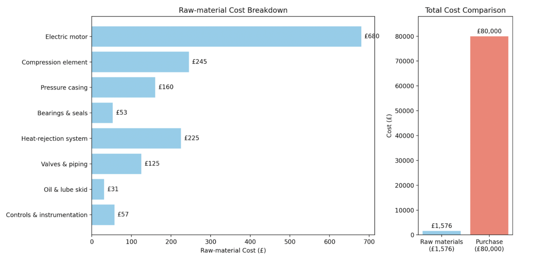
This gives us an >50x Idiot index! If we are to reduce capex at >20%, then we can’t afford this. To combat this level of inefficiency in the supply chain to aggressively come down the cost curve, we must vertically integrate all engineering and manufacturing.
However, we have to pick and choose our battles here. In some instances, supply and demand principles are working in our favour and actually produce a much cheaper product than we could if we in-housed engineering and manufacturing. With every process that is in-housed or removed as part of the reduction of the Idiot Index, you incur some level of complexity, resourcing and execution risk. This compounds quickly and suddenly without knowing you’ve spent all your R&D capital on a pump system that isn’t a core part of your IP. Therefore, there needs to be both a scale filter (e.g at what scale do we need to operate to make this vertical integration work?) and a market force filter (e.g at what scale is this part already produced, and how can we piggy-back on that?).
If you look through that lens, and look at the high-level BOM items in Carbon Engineering’s 2018 paper, you can plot those on a scale of cost vs global production to get something like this:

This immediately tells us to vertically integrate the top-left hand side of the graph, where the majority of the capex costs are concentrated and haven’t benefited from global production scale and cost reduction. Every step away from that corner we take, we should consider the complexity of bringing in-house vs purchasing off the shelf to take advantage of the already scaled production and cost reductions. After all, this 1.5kW 3-phase electric motor for £180 likely has an idiot index <3! Let’s make use of that.
Whilst vertical integration isn’t new, it often gets overlooked as a strategy because of the sheer complexity, capital intensiveness and execution risk. It’s really therefore a trade-off of complexity now and ease later, vs ease now and complexity later.
One direct outcome of vertical integration is the ability to control more variables that dictate the end cost of something. Since our entire focus is to reduce the levelised cost of capturing carbon, we must control as many variables that influence that cost as possible. In other words, we must increase the surface area available for us to achieve lower and lower costs. By outsourcing, you are essentially removing your ability to control costs, and thus are at the mercy of the market or individual suppliers. What if they increase their prices? What if they shut off your supply? Other than cost reduction, vertically integrating every step of the supply chains allows this level of control over costs. A good example of this is how SpaceX have been able to reduce the cost / kg to orbit:

This aggressive cost reduction was only possible by vertically integrating almost every component in a drive to reduce capex. At its core, it’s a reflection of isolating every variable that increased the cost of getting to orbit (namely, lack of reusability of rockets and bloated supply chains) and removing as constraints to come down the cost curve.
Focus on vertical integration to aggressively reduce capex also motivates towards simpler, more robust designs. If the aim is to reduce capex by 20% for every 0.25kWh of performance loss, this means aggressive cheap inefficiencies must be found! This is in contrast to an industry hellbent on squeezing that last bit of efficiency out of a system regardless of cost incurred. As we optimise for capex, simplicity and scalability, this immediately manifests in designs that on the surface seem counterintuitive. For example, if we want to decompose CaCO3 back to CaO, these would roughly be the options on a scale of cost vs efficiency:

Despite the incredible efficiencies of microwave and vacuum, the capex increase and the complexity in vertical integration immediately remove their attractiveness for more robust, age-old designs like resistive heating elements (after all, a toaster has fairly scaled manufacturing at this point).
Scaling these technologies
Driving down costs only really matters to the extent we can scale those designs. Lots of ground breaking R&D has performed well in a lab, but most never gets over the reality factor of building those creations in the real world at scale. Using numbers from earlier, we have 1200Gt of CO2 to remove from the air. Which architectures can operate at that scale, and what are the limiting factors?
For example, if we assume the idealised working capacity of Amines is ~200kg/tonne, cycled every day (e.g 365*400kg/tonne) to give us a yearly working capacity of 73 tonnes CO2/tonne, we would need just >16 billion tonnes of Amines to capture the 1200Gt of CO2 in the air to get back to safe levels! With global production of Amines at just under 3,000,000 tonnes a year, if we assume all other global usages of Amines stops immediately and no further CO2 gets into the sky, it would take us >5000 years of current global production rates to deliver the volumes we would need! We’re going to need a bigger boat.
Whilst dramatic ramping of production isn’t impossible, that would require a lot of extra Ethylene and Ammonia! Since the volume of excess CO2 in the air is so breathtakingly large, the scale of solutions needs to be baked into the strategy from day 1.
Some DAC architectures exhibit better inherent scaling coefficients than others. We can estimate scale exponent based on the following:
\[
b \;=\; \frac{\ln\!\left(\dfrac{C_{2}}{C_{1}}\right)}
{\ln\!\left(\dfrac{S_{2}}{S_{1}}\right)}.
\]
Where:
S1: the original capacity
C1: the cost at that original capacity
S2: the new (doubled) capacity
C2: the cost at the new capacity
From there, we’ll get a value (b) that gives us an idea of how well these architectures might scale:
| Architecture | Scale Exponent b |
Scaling Quality | Rationale & Scalability Details |
|---|---|---|---|
| KOH + Ca-Loop | 0.50 – 0.60 | Very Good | • Huge continuous vessels (absorber towers, precipitation basins, clarifiers) > CapEx grows sub-linearly. • Single large kilns/calciners can exceed 100 MW, driving b toward 0.5. • Shared utilities (steam, power, reagent recycle) serve all trains—dilutes fixed costs. • Heat integration (HRSG, slaker, turbine) further spreads Opex. |
| CaO Looping | 0.60 – 0.80 | Good – Moderate | • Calciner scales like petro/cement kilns (b≈0.6–0.7). • Air-contact beds stay modular (10–50 kt CO2 yr per module) > b drifts toward 0.8. • Pellet reactors, filters, transfer lines centralise, but solids-handling limits diameter. • Steam cycle & ASU gain from scale (b~0.6) only if co-located at large plants. |
| Solid-Amine TSA | 0.80 – 0.90 | Weak | • “Cartridge” format: hundreds of small beds in parallel. Minimal CapEx drag-down. • Heat/steam headers & blower skids upsize, but each bed still needs its own piping & valves. • Fan & heater banks gain modestly (b~0.7); bed count & adsorbent volume grow nearly linearly (b~1.0). |
| Zeolite (PSA/TSA) | 0.90 – 1.00 | Minimal | • Modular towers (<1 kt CO₂ yr each) cannot be economically widened much. • Compression/vacuum pumps & heat-exchange loops gain some scale (b~0.7), but adsorbent & vessel count dominate. • Skid-mount design: added capacity mostly means “more skids,” so cost grows almost linearly with throughput. |
What this shows is that the simpler architectures that are less efficient, have a much greater ability to scale in-the-limit vs those more performant options such as Amines and Zeolites. This is mostly based on (1) thermal decomposition with a kiln has very well understood scaling efficiencies from petro/cement industries, and (2) gas-solid contactor designs have no natural limiting factor, meaning in both instances raw materials are scaled more effectively where production/manufacturing is spread over a larger base. The same can’t be said for the other architectures, where the sorbents and vessel count dominate overall systems costs, and where scaling those is almost linear (e.g more of the same skid).
Distribution and utilisation
When we’ve worked so hard to capture it, what do we then do with it? We essentially have 2 choices – we either compress, store and inject underground (permanent removal), or we utilise for another product or process (utilisation). It’s important to not forget that CO2 is mostly only valuable to the extent that it’s used for other processes, and that if the CO2 in the sky was valuable, it would be harvested like every other resource on earth long ago. Reducing the cost of getting it out of the sky and into a high-productivity process is our route to making that true.
Although the main variables to consider are cost of the specific distribution or utilisation pathway, scale of that route-to-market, and price-point we’re selling the CO2 for, the underlying question is:
What is the fastest and cheapest route to a scaled market where there is sufficient profit head-room and access to capital whereby we can invest the profits rapidly to support increased R&D for further scaled deployment and reduction of the cost of capturing more Carbon Dioxide?
The current status-quo for DAC is storage > compression > injection underground and subsequent sale of credits. This is problematic based on the OPEX contribution as a % of levelised cost of CO2 is high, somewhere in the regime of 10-20%. This could therefore could add between £20 and £100/tonne assuming a total cost of CO2 capture between £500 and £100/tonne:

Alongside this, a credit-based system to sell the CO2 essentially means customers have to now pay for something they previously didn’t, and get nothing in return (e.g previously their emissions weren’t priced in). As such, there will always be push-back against this, as it doesn’t offer clear marginal utility to the customer.
Carbon-credits are also based on a fairly transient policy-market, meaning pricing and support can change rapidly. This limits access to large-scale project finance for these DAC projects, as institutional funders are looking for well-known markets where they can fund projects for 15-20 years with clear and concrete revenue structures, such as solar farms or toll roads.
For DAC companies, this means they have little certainty of future revenue prospects, lack of large-scale debt financing access, and are spending up to 20% of COGS on a process of getting their product underground that offers little to no utility for customers. In an ideal world, we would flip each of these issues, to look a little more like operating with future revenue certainty from well understood markets, access to large-scale infrastructure funding, and extremely small contributions to distribution as a % of COGS. What are the options for this?
| Pathway | High Sale Price | Large Market Size | Well-Understood Market | Low Access Costs | Total |
|---|---|---|---|---|---|
| Permanent geologic storage (saline aquifer or depleted field) |
5 | 6 | 6 | 6 | 23 |
| In-situ mineralisation (Carbfix-type basalt) |
5 | 5 | 5 | 6 | 21 |
| Ex-situ mineralised building products (CarbonCure, Blue Planet) |
8 | 7 | 5 | 5 | 25 |
| Synthetic fuels (e-jet, e-methanol, e-methane) |
8 | 9 | 9 | 8 | 34 |
| Commodity chemicals & polymers (urea, methanol, polyols) |
7 | 9 | 9 | 8 | 33 |
| Food- & beverage-grade CO₂ / dry ice | 8 | 7 | 8 | 3 | 26 |
| Novel consumer products (diamonds, carbon fibre, graphene) |
9 | 3 | 3 | 2 | 17 |
Qualitative grading is based on a scale of 1-10, with 10 being the best in each scenario. If we are to drive towards the cheapest capture of a CO2 molecule, the immediate valorisation of the raw molecule (e.g no drying requirement, little pressure requirement, and no scrubbing/polishing) with as few processes as possible is extremely important. The front runners offer that potential from the table are fuels & chemicals.
Fuels and chemicals are 2 of the largest markets on earth, with extremely well understood debt funding paths and global utility. The challenge is, and has always been, the ability to compete with these commodity markets on price. What that really means is the price of overcoming the thermodynamic barriers of H2 production and CO2 capture has been higher than the cost of drilling the ground. This was true in the world of the past where electrons cost >£0.5/kWh, but ceases to matter with the arrival of too-cheap-to-meter DC solar and aggressive vertical integration of all processes.
If we extrapolate almost any time in the future, chemically identical but carbon-neutral molecules will make-up the vast majority of all chemicals and fuel used on earth. This both provides an immediate valorisation pathway for DAC, but also a massive industry that will accelerate further deployments. This shift will become even more evident when batteries continue down their cost curve to electrify almost all industries, bar the following:
- Cement – High heat duty, with inherent CO2 offgas from limestone.
- Steel – H2/CO required for reduction of Iron Ore
- Long-haul Aviation – Batteries are significantly too heavy!
- Chemicals – CO2 and H2 required as feedstocks for ethylene, propylene, aromatics, methanol and others.
For these industries, there is either an energy-density challenge too great for batteries, or a molecular feedstock requirement that you can’t replace with an electron. They will become the bedrock of market opportunities for DAC to drive down the cost-curve and access vast financing options.
How does this all fit together?
Whichever way we look at the mechanisms to drive DAC costs lower, we are ultimately against the clock. The longer we wait, the worse things get, and the more we have to catch-up. Everything discussed is designed with a single goal: to accelerate DAC’s learning rate to the extent that it’s cheap enough to capture all carbon sources on earth.
Taking all deployments over the last 10 years, we get this:
| Year | New Capturing Ability Added (kt CO₂ yr⁻¹) |
Aggregate Volume Captured (kt CO₂ yr⁻¹) |
Price ($ t⁻¹) |
Notes |
|---|---|---|---|---|
| 2015 | 1.0 | 1.0 | 1 000 | Carbon Engineering pilot, Squamish (1 tonne day = 0.365 kt yr) |
| 2016 | 0.0 | 1.0 | 1 000 | |
| 2017 | 1.0 | 2.0 | 1 000 | Climeworks Hinwil (0.9 kt yr) + Hellisheiði mineral-storage unit (0.05 kt yr) |
| 2018 | 4.0 | 6.0 | 950 | Global Thermostat Huntsville pilot (up to 4 kt yr) |
| 2019 | 0.5 | 6.5 | 800 | Climeworks incremental expansions (~0.5 kt yr) |
| 2020 | 0.5 | 7.0 | 700 | Additional Climeworks capacity; learning-curve savings |
| 2021 | 2.0 | 9.0 | 600 | Climeworks + Global Thermostat add ≈2 kt yr |
| 2022 | 5.0 | 14.0 | 500 | Orca (4 kt yr⁻¹) and other builds accelerate growth |
| 2023 | 20.0 | 34.0 | 400 | 1PointFive pilots and other plants add ≈20 kt yr |
| 2024 | 50.0 | 84.0 | 300 | Mammoth (36 kt yr) and other large projects |
2025 hasn’t been added as we still have 6 months to go, but would accelerate these numbers with the planned commissioning of the 500Kt/yr Stratos. Using the numbers we have, there have been ~6 doublings over the last 10 years:
\[
\text{Doublings} \;=\;
\log_{2}\!\Bigl(\frac{84}{1}\Bigr)
\;\approx\;
\log_{2}(84)
\;\approx\; 6.4
\]
For every doubling, there was a ~ 13% price drop:
\[
\log(\mathrm{Price}) \;=\; a \;+\; b\,\log(\mathrm{Capacity})
\]
For every 13% price drop, it took ~ 1.8 years to happen:
\[
\text{Average Years per Doubling}
\;=\;
\frac{\displaystyle\sum_i \bigl(\text{Time between Doublings}\bigr)_i}
{\text{Number of Intervals}}.
\]
If we maintain that, and extrapolate to 2050, we get to £36/tonne – not bad!

What’s the impact if we influence the velocity of those learning rates (e.g time between doublings) both on the price and the aggregate captured tonnage, and the magnitude of those price reductions?
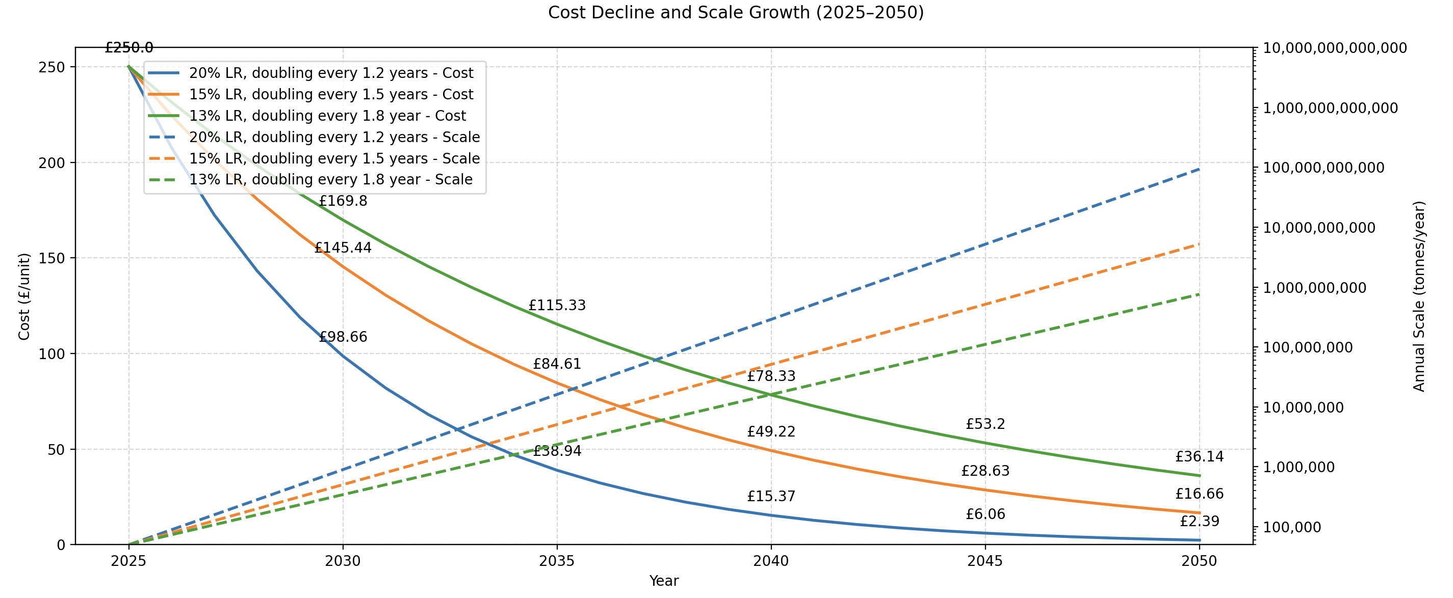
The green line represents our current path, ending with 1b tonnes removed annually by 2050. This is a strong start, but still only counts for 1Gt out of the 1200Gt we need to remove. Tweaking that rate to 15% vs 13%, and reducing doubling timeframe to 1.5 years, we get close to 10b tonnes/yr, and dip <£20/tonne by 2050.
The real kicker is the blue line. 20% cost reduction every 1.2 years, gets us to the heft 100b tonnes/year, meaning it would take just 10 years to remove 1200Gt in the air. This is what we’re after and must drive towards. This rate looks insane from where we are today, but we must not forget this level of price reduction isn’t new. The early feed-in tariffs for solar, like those in Germany and Japan in the early 2000’s, incentivised producers to export solar energy to the grid at pricing between €0.5 – 0.7/kWh, at a time when panels cost $5-6/watt (!). 25 years later, many panels retail for $0.06-0.08/watt, representing a 100x (99%) cost decrease. This can be replicated with DAC. For more analysis on how solar got cheap, see this blog.
This should go to show that we need all hands on deck to drive this learning rate forward to maintain the health of the planet. To give ourselves a fighting chance to forge that future into reality, these are the things that matter:
- Drive towards DAC architectures that exhibit the following:
- Low in complexity, robust in operation
- High in energy consumption and low in CAPEX, to benefit from the falling cost of solar energy
- Vast scaling coefficients in engineering and operation
- Ignore all advice that speaks to high efficiency and cutting edge science being the only architecture that works. This only mattered in a high-energy cost era.
- Vertically integrate all aspects of the process, from designing almost all components through to manufacturing and deployment. A >20% learning rate can’t afford to outsource much, nor the lead times that are deemed standard.
- Cheat the system by selling other products that use the captured carbon as an input material to access scalable capital markets, and show clear financial viability
- Act as a catalyst for larger, more impactful markets to adopt the technology to accelerate scale and cost reduction
Much like producing H2, we have a choice. We either fight the thermodynamics, or we fight the engineering. The same is true here with DAC. This reflects Rivan’s masterplan to reduce the CO2 in the air:
- Create a profit-bearing mechanism to capture CO2 from the air via synthetic fuels to halt net growth of CO2
- Use those synthetic fuels to decarbonise industries that cannot be electrified
- Continue to reduce the cost of CO2 capture to the extent we can capture all sources of CO2 profitably and sustainably
If you want to be part of that mission, get in touch ( harvey at rivan dot com) or apply to one of our open roles!